Apollo
Background
Apollo is a Genome Browser. It lets you visualize genes on a genome, create and edit genes, and create and edit annotations on those genes.
Genome Browsers are a vital tool for rapidly annotating genomes. They let you visualize multiple data sources and help you synthesize those into a rational set of annotations.
Definitions
- Static
- Unmodifiable. This is often used to refer to a set of “static” files made available over the web, or some other computer resource which cannot be modified. (Note that cannot be modified simply means that that exact file cannot be modified, but it is often possible to replace it with an updated version which is modified)
- Instance
- A specific copy of (usually) a web service made available over the internet. Given that the same web service could be duplicated and both could be accessible to users, we use the term “instance” to refer to a specific copy of a service.
- Credentials
- Username and password. Also may be used to mean an “API Key” which you can consider as a combined username and password
- Site
- This is sometimes used to mean your lab or organisation. Generally the people who have both deployed an Apollo instance for you, and you work with to annotate a genome.
GMOD, GBrowse, JBrowse, Apollo, what’s it all mean?
This section will be a bit of history about Genome Browsers, and while not important to the annotation process, it can be helpful to know what the terms means and how the parts all fit together.
We use a lot of software under the umbrella term of GMOD, the Generic Model Organism Database
The GMOD project collects open source software under a single umbrella, all related to the idea of publicly accessible, open source Model Organism Database (MOD). These are important, as historically every lab did their own thing. By having, at the very least, a common set of software for MODs, everyone could benefit from interoperability. Software that talked to one MOD could be re-used when talking to another MOD.
GBrowse
GBrowse was one of the earlier genome browsers, and continues to have wide popularity as it handles massive datasets quite well.
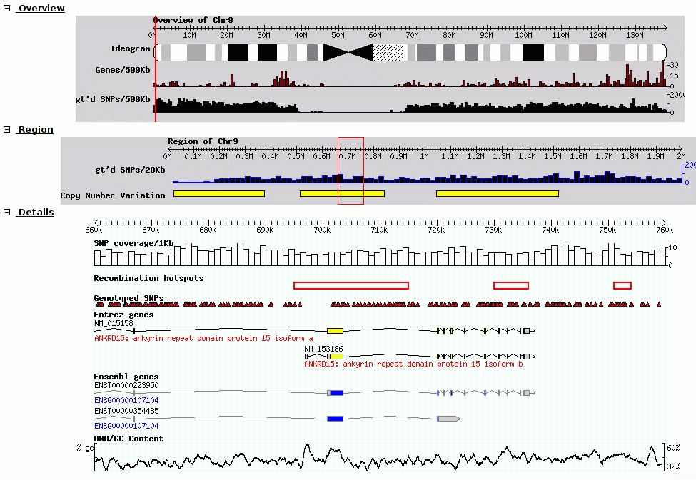
Fig. 25 Screenshot of GBrowse from GMOD Wiki
Tracks are rendered on the server, and the client view the genome and datasets through a set of static images shown to the user.
JBrowse
JBrowse and GBrowse are related and attempt to solve the same problem, JBrowse is a more modern, javascript version that does all of the processing on the client. This can make JBrowse much more responsive to user interactions, like how Google Maps was an improvement over previous web maps which required you to click and the page to refresh to load a new section of the map.
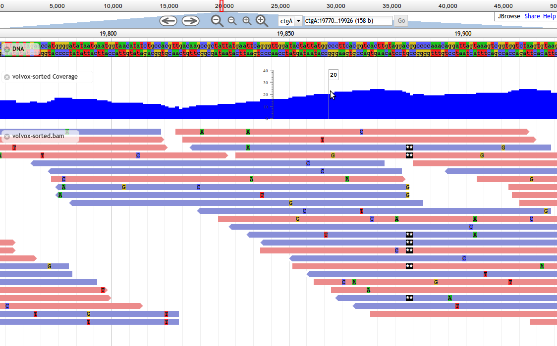
Fig. 26 Screnshot of a JBrowse instance. In this figure, JBrowse is shown displaying some alignments of sequencing reads to a genome. JBrowse has the ability to do things like dynamically colouring reads based on multiple properties, include read quality and direction.
Many labs have deployed JBrowse instances to help showcase their annotation efforts to the community, and to make their data accessible. Here you can see a demonstration of Drosophila melanogaster genes from FlyBase in JBrowse and play around with it.
Note that JBrowse is a static visualization tool, you cannot make any changes to the data, you cannot provide annotation and save them. It is a “Read Only” view of genomes and annotations.
Apollo
Apollo takes JBrowse one step further and adds infrastructure for community annotation; it provides a “Read+Write” view of genomes. You can create new gene features, new annotations on those features, and these are shared with everyone who has access to the Apollo server.
Apollo embeds JBrowse, so if you are familiar with JBrowse, many of the same skills apply.
Annotation File Formats
There are two formats you need to be aware of during genome annotation.
- Fasta, the format used to store DNA and protein sequences.
- GFF3, a widely used format for storing genome annotations.
- GenBank, an older format used by NCBI
Fasta
Many of you may have seen a fasta formatted sequence before, but briefly it looks like:
>phiX  Complete genome sequence of phage X
ACTGACTGATCGACTGCGTACGATCGACTGACT
CTGCGTACGATCGACTGACTACTGACTGATCGA
...
Each sequence starts with a >, and has a “fasta ID” after it. Some
sequences have a “description” after the sequence, like the in the above
“Complete genome...”
The sequences contained within a fasta file may be DNA, RNA, or protein sequences.
GFF3
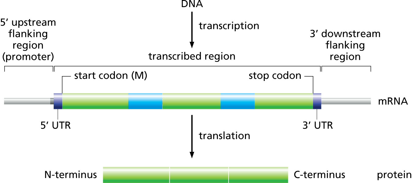
Fig. 27 This model is used by GFF3 and eukaryotic annotation efforts. Prokaryotic annotations may exhibit differences. Many organisations also use different standards and subsets of GFF3.
Many of you are probably familiar with the eukaryotic gene model. This model captures a lot of information about the biological process behind producing proteins from DNA, such as mRNAs, transcription, and alternative splicing. GFF3 files thus have to encode these complex, hierarchical, parent-child relationships.
Let’s look at what a GFF3 file looks like, briefly:
##gff-version 3.2.1
##sequence-region   ctg123 1 1497228
ctg123 . gene            1000  9000  .  +  .  ID=gene00001;Name=EDEN

ctg123 . mRNA            1050  9000  .  +  .  ID=mRNA00001;Parent=gene00001;Name=EDEN.1

ctg123 . exon            1201  1500  .  +  .  ID=exon00002;Parent=mRNA00001
ctg123 . exon            3000  3902  .  +  .  ID=exon00003;Parent=mRNA00001
ctg123 . exon            5000  5500  .  +  .  ID=exon00004;Parent=mRNA00001
ctg123 . exon            7000  9000  .  +  .  ID=exon00005;Parent=mRNA00001

ctg123 . CDS             1201  1500  .  +  0  ID=cds00001;Parent=mRNA00001;Name=edenprotein.1
ctg123 . CDS             3000  3902  .  +  0  ID=cds00001;Parent=mRNA00001;Name=edenprotein.1
ctg123 . CDS             5000  5500  .  +  0  ID=cds00001;Parent=mRNA00001;Name=edenprotein.1
ctg123 . CDS             7000  7600  .  +  0  ID=cds00001;Parent=mRNA00001;Name=edenprotein.1
And the visual representation of the text
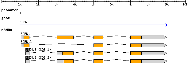
At the top level we see a “gene” (3rd column), which spans from 1000 to
9000, on the forward strand (7th column), with an ID of gene00001
and a Name of EDEN.
Below the gene, is an mRNA feature. We can infer that it is “below” in the
hierarchy based on the last column which has a Parent of gene00001.
Similarly all four exons and all four CDSs have a Parent of mRNA00001.
ID, Name, and Parent are all known as feature attributes.
Metadata about a feature. However, more information than just the names, IDs,
and relationships goes into feature attributes. Often you will see Notes,
sometimes Products, and many other tags besides. Only a couple of these
attributes have standards defining what information they contain, the rest are
free to be used as your organisation specifies, or as you like.
All of this is a little bit excessive for phages where real introns are rare, and mRNAs not involved, but nevertheless, we want to make sure our data is accessible to other researchers so they can do experiments building on our work.
(It is more important that you know the format exists, and that it encodes parent-child biological relationships, than that you know the precise specifics of what each column means.)
GenBank
In stark contrast to the elegance of the GFF3 format (tab separated, key-value pairs, easy to work with), we have the older GenBank format. This is a fixed-width format which has a “flat” gene model, and lacks any way to represent the hierarchical relationships that are biologically relevant.
LOCUS       NC_001133             230218 bp    DNA     linear   PLN 14-JUL-2011
DEFINITION  Saccharomyces cerevisiae S288c chromosome I, complete sequence.
ACCESSION   NC_001133
VERSION     NC_001133.9  GI:330443391
DBLINK      Project: 128
KEYWORDS    .
SOURCE      Saccharomyces cerevisiae S288c
  ORGANISM  Saccharomyces cerevisiae S288c
            Eukaryota; Fungi; Dikarya; Ascomycota; Saccharomycotina;
            Saccharomycetes; Saccharomycetales; Saccharomycetaceae;
            Saccharomyces.
REFERENCE   1  (bases 1 to 230218)
  AUTHORS   Goffeau,A., Barrell,B.G., Bussey,H., Davis,R.W., Dujon,B.,
            Feldmann,H., Galibert,F., Hoheisel,J.D., Jacq,C., Johnston,M.,
            Louis,E.J., Mewes,H.W., Murakami,Y., Philippsen,P., Tettelin,H. and
            Oliver,S.G.
  TITLE     Life with 6000 genes
  JOURNAL   Science 274 (5287), 546 (1996)
   PUBMED   8849441
FEATURES             Location/Qualifiers
     source          1..230218
                     /organism="Saccharomyces cerevisiae S288c"
                     /mol_type="genomic DNA"
                     /strain="S288c"
                     /db_xref="taxon:559292"
                     /chromosome="I"
     gene            complement(1807..2169)
                     /gene="PAU8"
                     /locus_tag="YAL068C"
                     /db_xref="GeneID:851229"
     mRNA            complement(<1807..>2169)
                     /gene="PAU8"
                     /locus_tag="YAL068C"
                     /transcript_id="NM_001180043.1"
                     /db_xref="GI:296142466"
                     /db_xref="GeneID:851229"
     CDS             complement(1807..2169)
                     /gene="PAU8"
                     /locus_tag="YAL068C"
                     /note="hypothetical protein, member of the seripauperin
                     multigene family encoded mainly in subtelomeric regions"
                     /codon_start=1
                     /protein_id="NP_009332.1"
                     /db_xref="GI:6319249"
                     /db_xref="SGD:S000002142"
                     /db_xref="GeneID:851229"
...
ORIGIN
        1 ccacaccaca cccacacacc cacacaccac accacacacc acaccacacc cacacacaca
       61 catcctaaca ctaccctaac acagccctaa tctaaccctg gccaacctgt ctctcaactt
There are a few major regions of a GenBank file:
- The header (Starting with LOCUS...)
- The feature table (Starting with FEATURES)
- The sequence
The header will tell you information like:
- Sequence ID, NC_001133 in the above example,
- Genome or chromosome length
- Annotation set version (9, from
VERSION NC_001133.9) - References
The feature table usually starts with a “source” type feature which
contains metadata about the chromosome or genome. Features consist of a
feature type key on the left, and key value pairs on the right formatted
as /key="Value...".
Lastly, there is the sequence data. In contrast to GFF3 which stores sequence data in standardised fasta format, GenBank uses sequence separated into six columns of ten characters, with the sequence index annotated on the left.
Annotation
On to actually using Apollo! We’ll go through an example annotation.You’re welcome to follow along with this at home and familiarize yourself with Apollo before class. The example presented here will be open for everyone in the class to use, so images may not reflect the current annotations made.
There are two primary components to an annotation pipeline:
- Structural annotation
- Functional annotation
In structural annotation you will likely take the output of gene callers, and perhaps other evidence tracks, and use these results to annotate putative genes in Apollo. Structural annotations consist of locations of genomic features, like genes, terminators, and tRNAs.
Functional annotation will entail identifying possible gene functions based on different evidence sources. We will go into more detail in the first lecture on what it means to do structural and functional annotations.
Apollo in Galaxy
This section will cover the generalised use of Apollo in Galaxy, not specific to any annotation workflow implementation.
Fig. 28 This error might appear, from time to time. It is safe to ignore.
Registration
In order to log in to Apollo, you’ll need to register for an account using the Galaxy tool, if your site has not already set up one for you.

In the integrated Galaxy-Apollo workflow, you can register for an account by running a Galaxy tool, which will generate your credentials for you. If you ever forget your credentials and cannot find the item in your history, you can re-run this, and it will generate a new password for you.
Simply fill out the form:
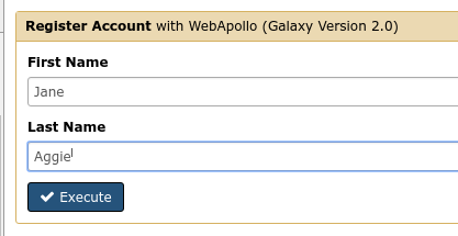
And hit the Execute button. Once the tool is done running, the dataset will turn green. You will then click the “View Dataset” eyeball button to see your password. (You don’t need to memorize this password or write it down anywhere. You can always come back to Galaxy to view it.)
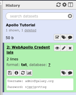
Fig. 29 If you ever lose your Galaxy history with the password, just come back to Galaxy and re-run the tool. The password will be saved there for you.
JBrowse In Galaxy
If you’re familiar with JBrowse, a view of Apollo should look familiar to you:
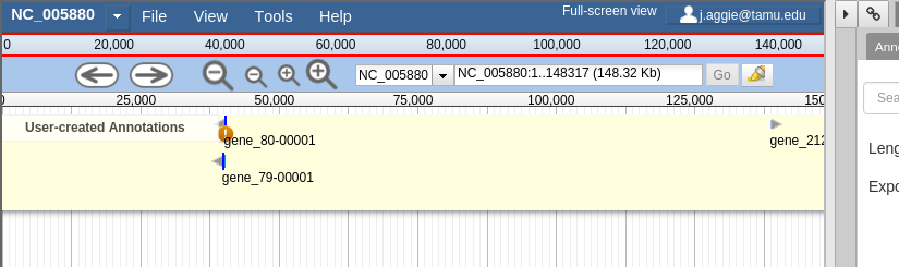
Fig. 30 Notice the JBrowse window embedded within the Apollo interface. Apollo integrates with the JBrowse software to provide the ability to make annotations and save them.
The CPT developed a tool called JBrowse-in-Galaxy (JiG) which allows you to build JBrowse instances within Galaxy. JBrowse instances are traditionally configured through a complex and manual process at the command line. JiG represents the first ever visual JBrowse configuration and construction tool.
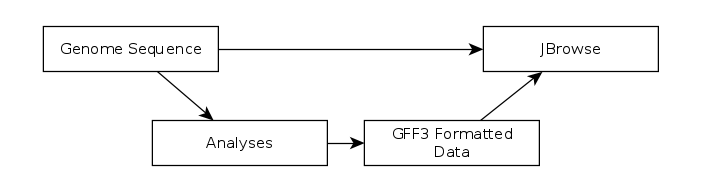
Fig. 31 The generalized JBrowse workflow. JBrowse is simply a tool for displaying the results of a bioinformatic analysis in a standardised way.
Apollo takes, as its input, complete JBrowse instances. To view any data in Apollo, a JBrowse instance needs to be configured first.
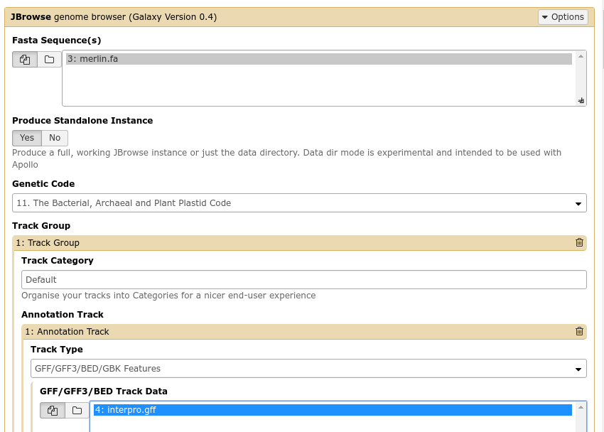
Fig. 32 The JBrowse-in-Galaxy tool is an extremely complex tool, with a very detailed manual (at the bottom of the page in Galaxy). If you need to do anything beyond showing simple GFF3 files, you’ll need to read this manual.
Once you’ve created a JBrowse instance, you’ll find it in your history
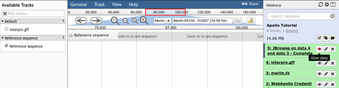
Fig. 33 Viewing a JBrowse instance produced within Galaxy.
If you chose to produce a “standalone instance,” you’ll be able to click the eyeball icon and view the dataset.
Moving Data from Galaxy to Apollo
Now that you have:
- A complete JBrowse instance
- Apollo credentials
You’re ready to start talking to the Apollo service.
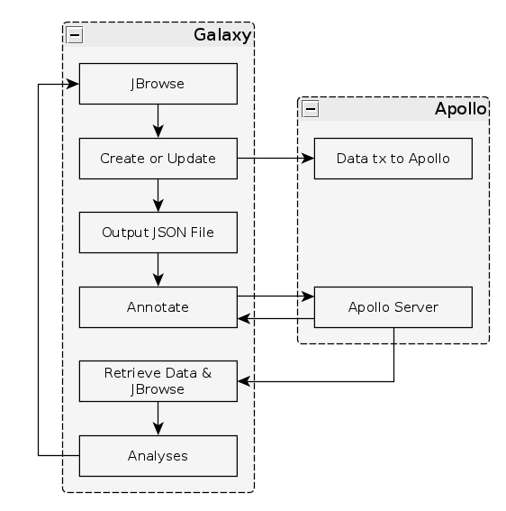
Fig. 34 The general Apollo/JiG/Galaxy workflow. Data is built up in Galaxy in the form of a JBrowse instance, which is pushed to the Apollo service in the Create or Update step, and transfers data to Apollo. The Annotate step is simple a convenience method for accessing Apollo. Apollo is also available at https://your-organisations-galaxy-instance/apollo. These methods both point at the same instance of Apollo.
The first tool we’ll use is a tool named Create or Update which lets us create, or update, an organism in Apollo with new data from Galaxy in the form of a JBrowse instance.
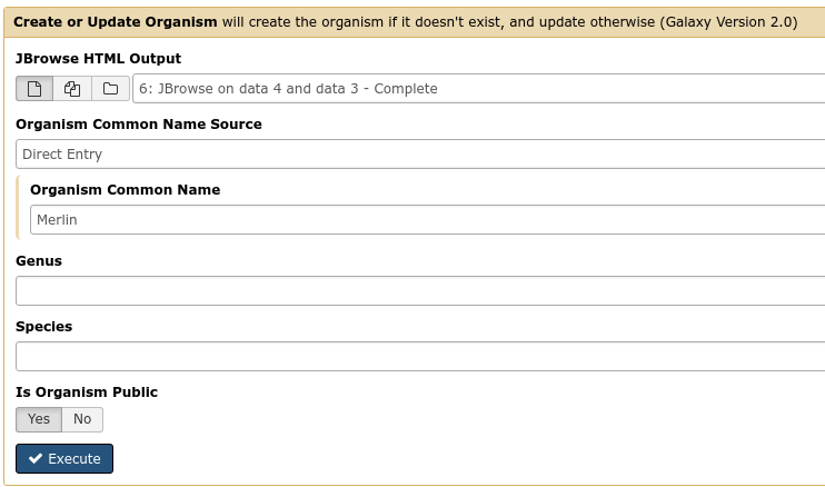
Fig. 35 It is not required (but highly recommended) to fill out the species field appropriately. Additionally it is not required to make anything public (available to the public at large) but it is encouraged.
This step will transfer data to Apollo, and produce a JSON file. The output JSON file contains some metadata about the organism. You will never need any information from this file.
Now that your data is available in Apollo, you can access it at Apollo, or via the Annotate convenience method which is provided. The Annotate tool takes the JSON file from a Create or Update step, and loads Apollo, directly in Galaxy.
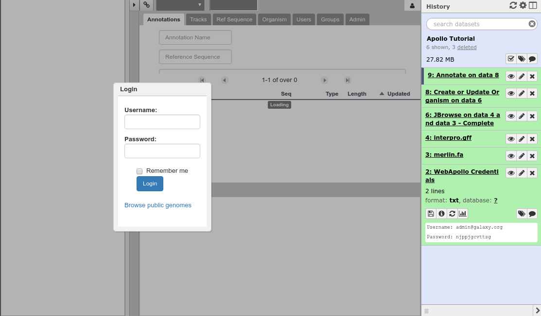
Fig. 36 Apollo accessed from within Galaxy
Finding Our Way Around
You’ll be presented with a two-pane display. On the left is an embedded JBrowse instance:
Fig. 37 JBrowse is a key component of Apollo. Apollo adds some additional options to JBrowse’s top menu, and the pale yellow track labeled “User-created Annotations”
JBrowse, embedded in Apollo, is slightly different than a normal JBrowse. The movement controls are all the same:
- you can use the magnifying glasses to zoom in and out of the genome and its data
- the arrow icons will move you up and downstream along the genome
- Selecting or clicking on locations along the genome ruler (they grey box at the top of the genome, 0 bp; 20,000bp; 40,000bp; etc.) will allow you to zoom in and move to specific regions
The menu bar has some useful options, some that aren’t available in “standard” JBrowse:
- File allows adding some special track types. We will not be using these options, but it’s recommended that you explore them.
- View will let you set some useful options:
- “Color by CDS frame” is a popular option during annotation. It will colour each coding sequence by which frame the reading frame is in.
- “Show Track Label” is an incredibly useful feature to hide the track’s labelling, allowing you to annotate small features near the end of the genome, which would otherwise be hidden by the track label (E.g. “User created annotations”)
The pale yellow track that is visible is the User Created Annotation track. During the annotation of a genome, gene features will be added to this track and edited, thus this track will always be visible to you.
Back to the overview ,on the right is the Genome Selector, which lists all of the organisms accessible to you.
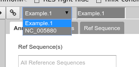
Fig. 38 Apollo uses the concept of “Organisms” with “reference sequences” below it. Each organism can have one or more reference sequences. In higher order organisms those often correspond to multiple chromosomes. For phage uses they are most often used to correspond to different assemblies of the genome.
The Ref Sequence tab lists all of the sequences (associated with a given organism) that are accessible to you.
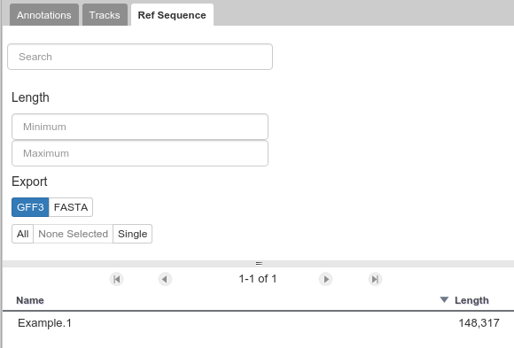
Fig. 39 This panel allows you to switch between reference sequences and filter them (in the event that there are many reference sequences).
For those familiar with JBrowse, you will notice that the track selection menu is missing. You will find it under the Tracks tab on the right hand side.
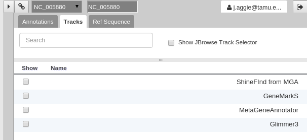
Fig. 40 Track Selection
If you select all three of the tracks (GeneMarkS, MetaGeneAnnotator, and Glimmer3), they will show up in JBrowse. You may find that this produces an absolutely overwhelming amount of information:
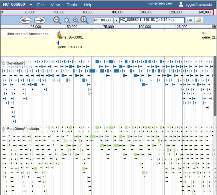
Fig. 41 Overwhelming
In order to combat that, you should zoom in
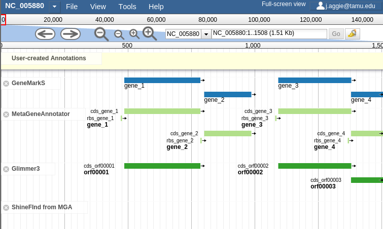
Fig. 42 Zooming
You may find that you wish to focus solely on the annotation process, without any distractions from the Apollo portion of the interface. You can hide that easily.
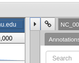
Fig. 43 Hiding Apollo
Let’s zoom down to the level of a single gene:
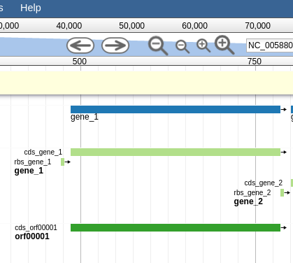
Fig. 44 Here we can begin to compare the gene models of these three genes. One of the three has a Shine Dalgarno sequence anotated. The CPT filters all SD sequences to ensure that only high quality ones are visible.
Great! Here we see the very first gene called by the three gene callers that we use.
Note
Your work is saved automatically, instantaneously. You do not need to worry about losing changes.